Topics
Mathematical Reasoning
- Mathematically Acceptable Statements
- New Statements from Old
- Special Words Or Phrases
- Contrapositive and Converse
- Introduction of Validating Statements
- Validation by Contradiction
- Difference Between Contradiction, Converse and Contrapositive
- Consolidating the Understanding
Sets
- Sets and Their Representations
- Empty Set (Null or Void Set)
- Finite and Infinite Sets
- Equal Sets
- Subsets
- Power Set
- Universal Set
- Venn Diagrams
- Intrdouction of Operations on Sets
- Union of Sets
- Intersection of Sets
- Difference of Sets
- Complement of a Set
- Practical Problems on Union and Intersection of Two Sets
- Proper and Improper Subset
- Open and Close Intervals
- Disjoint Sets
- Element Count Set
Sets and Functions
Relations and Functions
- Cartesian Product of Sets
- Concept of Relation
- Concept of Functions
- Some Functions and Their Graphs
- Algebra of Real Functions
- Ordered Pairs
- Equality of Ordered Pairs
- Pictorial Diagrams
- Graph of Function
- Pictorial Representation of a Function
- Exponential Function
- Logarithmic Functions
- Brief Review of Cartesian System of Rectanglar Co-ordinates
Algebra
Trigonometric Functions
- Concept of Angle
- Introduction of Trigonometric Functions
- Signs of Trigonometric Functions
- Domain and Range of Trigonometric Functions
- Trigonometric Functions of Sum and Difference of Two Angles
- Trigonometric Equations
- Trigonometric Functions
- Truth of the Identity
- Negative Function Or Trigonometric Functions of Negative Angles
- 90 Degree Plusminus X Function
- Conversion from One Measure to Another
- 180 Degree Plusminus X Function
- 2X Function
- 3X Function
- Expressing Sin (X±Y) and Cos (X±Y) in Terms of Sinx, Siny, Cosx and Cosy and Their Simple Applications
- Graphs of Trigonometric Functions
- Transformation Formulae
- Values of Trigonometric Functions at Multiples and Submultiples of an Angle
- Sine and Cosine Formulae and Their Applications
Coordinate Geometry
Complex Numbers and Quadratic Equations
- Concept of Complex Numbers
- Algebraic Operations of Complex Numbers
- The Modulus and the Conjugate of a Complex Number
- Argand Plane and Polar Representation
- Quadratic Equations
- Algebra of Complex Numbers - Equality
- Algebraic Properties of Complex Numbers
- Need for Complex Numbers
- Square Root of a Complex Number
Calculus
Mathematical Reasoning
Linear Inequalities
Principle of Mathematical Induction
Statistics and Probability
Permutations and Combinations
- Fundamental Principles of Counting
- Permutations
- Combination
- Introduction of Permutations and Combinations
- Permutation Formula to Rescue and Type of Permutation
- Smaller Set from Bigger Set
- Derivation of Formulae and Their Connections
- Simple Applications of Permutations and Combinations
- Factorial N (N!) Permutations and Combinations
Binomial Theorem
- Introduction of Binomial Theorem
- Binomial Theorem for Positive Integral Indices
- General and Middle Terms
- Proof of Binomial Therom by Pattern
- Proof of Binomial Therom by Combination
- Rth Term from End
- Simple Applications of Binomial Theorem
Sequence and Series
Straight Lines
- Slope of a Line
- Various Forms of the Equation of a Line
- General Equation of a Line
- Distance of a Point from a Line
- Brief Recall of Two Dimensional Geometry from Earlier Classes
- Shifting of Origin
- Equation of Family of Lines Passing Through the Point of Intersection of Two Lines
Conic Sections
- Sections of a Cone
- Concept of Circle
- Introduction of Parabola
- Standard Equations of Parabola
- Latus Rectum
- Introduction of Ellipse
- Relationship Between Semi-major Axis, Semi-minor Axis and the Distance of the Focus from the Centre of the Ellipse
- Special Cases of an Ellipse
- Eccentricity
- Standard Equations of an Ellipse
- Latus Rectum
- Introduction of Hyperbola
- Eccentricity
- Standard Equation of Hyperbola
- Latus Rectum
- Standard Equation of a Circle
Introduction to Three-dimensional Geometry
Limits and Derivatives
- Intuitive Idea of Derivatives
- Introduction of Limits
- Introduction to Calculus
- Algebra of Limits
- Limits of Polynomials and Rational Functions
- Limits of Trigonometric Functions
- Introduction of Derivatives
- Algebra of Derivative of Functions
- Derivative of Polynomials and Trigonometric Functions
- Derivative Introduced as Rate of Change Both as that of Distance Function and Geometrically
- Limits of Logarithmic Functions
- Limits of Exponential Functions
- Derivative of Slope of Tangent of the Curve
- Theorem for Any Positive Integer n
- Graphical Interpretation of Derivative
- Derive Derivation of x^n
Statistics
- Measures of Dispersion
- Concept of Range
- Mean Deviation
- Introduction of Variance and Standard Deviation
- Standard Deviation
- Standard Deviation of a Discrete Frequency Distribution
- Standard Deviation of a Continuous Frequency Distribution
- Shortcut Method to Find Variance and Standard Deviation
- Introduction of Analysis of Frequency Distributions
- Comparison of Two Frequency Distributions with Same Mean
- Statistics Concept
- Central Tendency - Mean
- Central Tendency - Median
- Concept of Mode
- Measures of Dispersion - Quartile Deviation
- Standard Deviation - by Short Cut Method
Probability
- Random Experiments
- Introduction of Event
- Occurrence of an Event
- Types of Events
- Algebra of Events
- Exhaustive Events
- Mutually Exclusive Events
- Axiomatic Approach to Probability
- Probability of 'Not', 'And' and 'Or' Events
Notes
Axiomatic approach is another way of describing probability of an event. In this approach some axioms or rules are depicted to assign probabilities.
It follows from the axiomatic definition of probability that
(i) `0 ≤ P (ω_i) ≤ 1 "for each" ω_i ∈ S `
(ii) `P (ω_1) + P (ω_2) + ... + P (ω_n)` = 1
(iii) For any event A, `P(A) = ∑ P(ω_i ), ω_i ∈ A.`
For example, in ‘a coin tossing’ experiment we can assign the number `1/2` to each of the outcomes H and T.
i.e. P(H) = `1/2` and and P(T) = `1/2` ...(1)
The both the conditions i.e., each number is neither less than zero nor greater than 1 and
P(H) + P(T) = `1/2 +1/2` = 1
Therefore, in this case we can say that probability of H = `1/2` , and probability of
T = `1/2`
If we take P(H) = `1/4` and P(T) = 3/4 ...(2)
We find that both the assignments (1) and (2) are valid for probability of H and T. In fact, we can assign the numbers p and (1 – p) to both the outcomes such that 0 ≤ p ≤ 1 and P(H) + P(T) = p + (1 – p) = 1
This assignment, too, satisfies both conditions of the axiomatic approach of probability.
1) Probability of an event :
Let S be a sample space associated with the experiment ‘examining three consecutive pens produced by a machine and classified as Good (non-defective) and bad (defective)’.
For example:
A sample space associated with this experiment is
S = {BBB, BBG, BGB, GBB, BGG, GBG, GGB, GGG},
where B stands for a defective or bad pen and G for a non – defective or good pen.
Let the probabilities assigned to the outcomes be as follows
| Sample point | BBB | BBG | BGB | GBB | BGG | GBG | GGB | GGG |
| Probability | `1/8` | `1/8` | `1/8` | `1/8` | `1/8` | `1/8` | `1/8` | `1/8` |
Let event A: there is exactly one defective pen and event B: there are atleast two defective pens.
Hence A = {BGG, GBG, GGB} and
B = {BBG, BGB, GBB, BBB}
Now P(A) = P(BGG) + P(GBG) + P(GGB) = `1/8 + 1/8 +1/8 = 3/8`
and P(B) = P(BBG) + P(BGB) + P(GBB) + P(BBB) = `1/8+1/8+1/8+1/8 = 4/8 = 1/2`
2) Probabilities of equally likely outcomes:
Let a sample space of an experiment be
`S = {ω_1, ω_2,..., ω_n}.`
Let all the outcomes are equally likely to occur, i.e., the chance of occurrence of each simple event must be same. i.e.
`P(ω_i)` = p, for all `ω_i` ∈ S where 0 ≤ p ≤ 1
Since \[\displaystyle\sum_{i=1}^{n} P(\omega_i) \] = 1
i.e., p + p +...+ p (n times) = 1
or np = 1 i.e., p = 1/n
Let S be a sample space and E be an event, such that n(S) = n and n(E) = m. If each out come is equally likely, then it follows that
P(E) = `m/n = ("Numberof outcomes favourable to E")/ ("Total possible outcomes")`
3) Probability of the event ‘A or B’:
Find the probability of event ‘A or B’, i.e., P (A ∪ B)
Let A = {HHT, HTH, THH} and B = {HTH, THH, HHH} be two events associated with ‘tossing of a coin thrice’
Clearly A ∪ B = {HHT, HTH, THH, HHH}
Now P (A ∪ B)
= P(HHT) + P(HTH) + P(THH) + P(HHH)
If all the outcomes are equally likely, then
`P(A U B) = 1/8 + 1/8 + 1/8 + 1/8 = 4/8 = 1/2`
Also P(A) = P(HHT) + P(HTH) + P(THH) = `3/8`
and P(B) = P(HTH) + P(THH) + P(HHH) = `3/8`
Therefore P(A) + P(B) =` 3/8 + 3/8 = 6/8`
It is clear that P(A∪ B) ≠ P(A) + P(B)
The points HTH and THH are common to both A and B. In the computation of P(A) + P(B) the probabilities of points HTH and THH, i.e., the elements of A ∩B are included twice. Thus to get the probability P(A∪B) we have to subtract the probabilities of the sample points in A ∩ B from P(A) + P(B)
i.e. P(A∪ B) = P(A)+ P(B) -
` P(ω_i ), ∀ ω_i ∈ A ∩ B `
= = P(A)+ P(B) - P( A ∩ B)
Thus we observe that, P(A ∪ B)= P(A)+ P(B)- P(A ∩ B).
Alternatively, it can also be proved as follows:
A ∪ B = A ∪ (B – A), where A and B – A are mutually exclusive,
and B = (A ∩ B) ∪ (B – A), where A ∩ B and B – A are mutually exclusive.
Using Axiom (iii) of probability, we get
P (A ∪B) = P (A) + P (B – A) ... (2) and
P(B) = P ( A ∩ B) + P (B – A) ... (3)
Subtracting (3) from (2) gives
P (A ∪ B) – P(B) = P(A) – P (A ∩ B) or
P(A ∪ B) = P(A) + P (B) – P (A ∩ B)
The above result can further be verified by observing the Venn Diagram Fig. 
If A and B are disjoint sets, i.e., they are mutually exclusive events, then A ∩ B = φ
Therefore P(A∩ B) = P ( φ) = 0
Thus, for mutually exclusive events A and B, we have
P(A∪ B)= P(A) + P(B),
which is Axiom(iii) of probability.
4) Probability of event ‘not A’ :
Consider the event A = {2, 4, 6, 8} associated with the experiment of drawing a card from a deck of ten cards numbered from 1 to 10. Clearly the sample space is S = {1, 2, 3, ...,10}
If all the outcomes 1, 2, ...,10 are considered to be equally likely, then the probability of each outcome is` 1/10`
Now P(A) = P(2) + P(4) + P(6) + P(8)
= `1/10 + 1/10 + 1/10 + 1/10 = 4/10 = 2/5`
Also event ‘not A’ = A′ = {1, 3, 5, 7, 9, 10}
Now P(A′) = P(1) + P(3) + P(5) + P(7) + P(9) + P(10)
`= 6/10 = 3/5`
Thus P(A') = `3/5 = 1-2/5` = 1- P(A)