Topics
Linear equations in two variables
- Introduction to linear equations in two variables
- Methods of solving linear equations in two variables
- Simultaneous method
- Simultaneous method
- Substitution Method
- Cross - Multiplication Method
- Graphical Method
- Determinant method
- Determinant of Order Two
- Equations Reducible to a Pair of Linear Equations in Two Variables
- Simple Situational Problems
- Pair of Linear Equations in Two Variables
- Application of simultaneous equations
- Simultaneous method
Quadratic Equations
- Quadratic Equations
- Roots of a Quadratic Equation
- Solutions of Quadratic Equations by Factorization
- Solutions of Quadratic Equations by Completing the Square
- Formula for Solving a Quadratic Equation
- Nature of Roots of a Quadratic Equation
- The Relation Between Roots of the Quadratic Equation and Coefficients
- To Obtain a Quadratic Equation Having Given Roots
- Application of Quadratic Equation
Arithmetic Progression
- Introduction to Sequence
- Terms in a sequence
- Arithmetic Progression
- General Term of an Arithmetic Progression
- Sum of First ‘n’ Terms of an Arithmetic Progressions
- Arithmetic Progressions Examples and Solutions
- Geometric Progression
- General Term of an Geomatric Progression
- Sum of the First 'N' Terms of an Geometric Progression
- Geometric Mean
- Arithmetic Mean - Raw Data
- Concept of Ratio
Financial Planning
Probability
- Probability - A Theoretical Approach
- Basic Ideas of Probability
- Random Experiments
- Outcome
- Equally Likely Outcomes
- Sample Space
- Event and Its Types
- Probability of an Event
- Type of Event - Elementry
- Type of Event - Complementry
- Type of Event - Exclusive
- Type of Event - Exhaustive
- Concept Or Properties of Probability
- Addition Theorem
Statistics
- Tabulation of Data
- Inclusive and Exclusive Type of Tables
- Ogives (Cumulative Frequency Graphs)
- Applications of Ogives in Determination of Median
- Relation Between Measures of Central Tendency
- Introduction to Normal Distribution
- Properties of Normal Distribution
- Concepts of Statistics
- Mean of Grouped Data
- Method of Finding Mean for Grouped Data: Direct Method
- Method of Finding Mean for Grouped Data: Deviation Or Assumed Mean Method
- Method of Finding Mean for Grouped Data: the Step Deviation Method
- Median of Grouped Data
- Mode of Grouped Data
- Concept of Pictograph
- Presentation of Data
- Graphical Representation of Data as Histograms
- Frequency Polygon
- Concept of Pie Graph (Or a Circle-graph)
- Interpretation of Pie Diagram
- Drawing a Pie Graph
Notes
The information in a frequency table can be presented in various ways. We have studied a histogram. A frequency polygon is another way of presentation.
Let us study two methods of drawing a frequency polygon.
(1) With the help of a histogram (2) Without the help of a histogram.
(1) We shall use the histogram in figure to learn the method of drawing a frequency polygon.

1. Mark the mid - point of upper side of each rectangle in the histogram.
2. Assume that a rectangle of zero height exists preceeding the first rectangle and mark its mid - point. Similarly, assume a rectangle succeeding the last rectangle and mark its mid -point.
3. Join all mid - points in order by line segments.
4. The closed figure so obtained is the frequency polygon.
(2) Observe the following table. It shows how the coordinates of points are decided to draw a frequency polygon, without drawing a histogram.

The points corresponding to the coordinates in the fifth column are plotted. Joining them in order by line segments, we get a frequency polygon. The polygon is shown in figure . Observe it.

Related QuestionsVIEW ALL [11]
The following table shows the average rainfall in 150 towns. Show the information by a frequency polygon.
|
Average rainfall (cm)
|
0 - 20 | 20 - 40 | 40 - 60 | 60 - 80 | 80 - 100 |
| No. of towns | 14 | 12 | 36 | 48 | 40 |
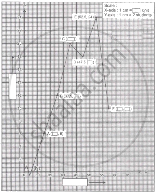
In the following frequency distribution, the heights of 90 students are recorded and the frequency polygon is drawn.
| Heights | 30 – 35 | 35 – 40 | 40 – 45 | 45 – 50 | 50 – 55 | 55 – 60 |
| No. of Students | 6 | 12 | 20 | 18 | 24 | 10 |
Draw a frequency polygon from the information given in the following table.
| Age of blood donar (Years) | No. of blood donars |
| Less than 20 | 0 |
| Less than 25 | 30 |
| 75Less than 30 | 75 |
| 165Less than 35 | 127 |
| Less than 40 | 165 |
| Less than 45 | 185 |
| Less than 50 | 197 |
The time required for students to do a science experiment and the number of students is shown in the following grouped frequency distribution table. Show the information by a histogram and also by a frequency polygon.
|
Time required for
experiment (minutes) |
20 - 22 | 22 - 24 | 24 - 26 | 26 - 28 | 28 - 30 | 30 - 32 |
| No. of students | 8 | 16 | 22 | 18 | 14 | 12 |
In a handloom factory different workers take different periods of time to weave a saree. The number of workers and their required periods are given below. Present the information by a frequency polygon.
|
No. of days
|
8 - 10 | 10 - 12 | 12 - 14 | 14 - 16 | 16 - 18 | 18 - 20 |
| No. of workers | 5 | 16 | 30 | 40 | 35 | 14 |
Draw a frequency polygon for the following grouped frequency distribution table.
|
Age of the donor
(Yrs.) |
20 - 24 | 25 - 29 | 30 - 34 | 35 - 39 | 40 - 44 | 45 - 49 |
| No. of blood doners | 38 | 46 | 35 | 24 | 15 | 12 |
The maximum bowing speed (km/hour) or 33 players at a cricket coaching centre is given below:
| Bowling Speed(km/hour) | 85-100 | 100-115 | 115-130 | 130-145 |
| Numbers of players | 9 | 11 | 8 | 5 |
find the modal bowling speed of players.
