Some Functions and Their Graphs

(i) Identity function- In this type of functions the value of x and f(x) is identical i.e same that's why it is known as Identity function. There are two ways to represent function they are Rule and Graph.
A function is represented in Rule like, if x=1 then f(x)=1
Graph- 

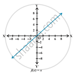
In indentical function if y=f(x) then y=x
We have already learnt that domain is a set of values of x at which function is defined. And for values of x at which function is defined, set of values of f(x) is called as Range.
Here, f(x)=x 
Domain= R
Range= R

(ii) Constant function- For any value of x, f(x) is always constant. f(x)= c is the constant function. 
Here, Domain= R and Range= {c}

The graph is a line parallel to x-axis. For example, if f(x)=3 for each x∈R, then its graph will be a line as shown in the Fig.

(iii) Polynomial function- A polynomial function is written as `f(x)= a_0+ a_1x+ a_2x^2+ a_3x^3+..... +a_nx^n`, where n is a non-negative integer and  `a_0, a_1, a_2,...,a_n∈"R".` 
There is no definite graph of a polynomial function. Say `f(x)=x^2`, draw the graph of f.

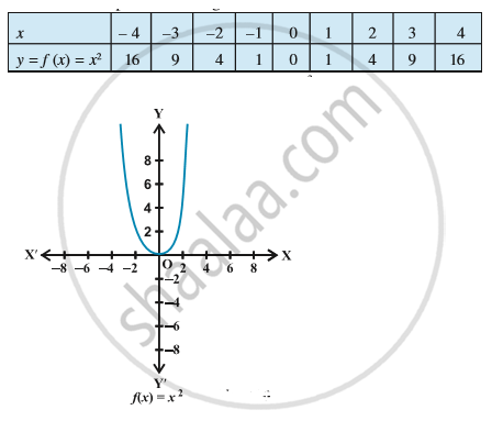
Here, `f(x)=x^2` can also be written as f: R→R
Domain= R and Range= `"R"^+`
Let's take another example, Draw the graph of the function f :R → R defined by `f (x) = x^3, x∈"R".`
f(0) = 0, f(1) = 1, f(–1) = –1, f(2) = 8, f(–2) = –8,  f(3) = 27; f(–3) = –27, etc. 

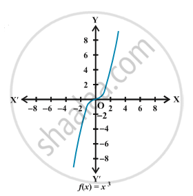
Here, `f(x)= x^3, f: "R"→"R"`
Domain= R and Range= R

(iv) Rational functions- Relation functions are of the type `f(x)= g(x)/[h(x)]≠ 0`
 Example- Define the real valued function f : R – {0}→ R defined by `f(x)= 1/x, x ∈ R -{0}`

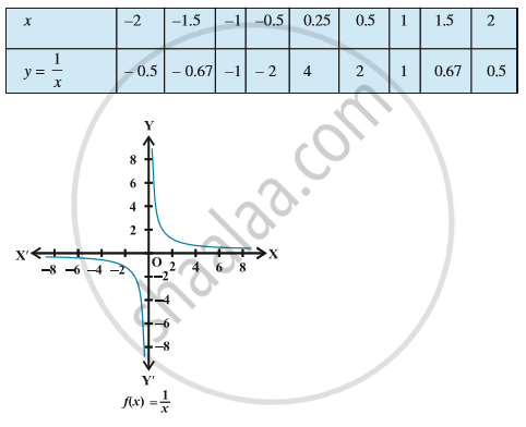
`f(x)=1/x`, Domain= R-{0} and Range= R-{0}

(v) The Modulus function- The function f: R→R defined by f(x) = |x| for each x ∈R is called modulus function. For each non-negative value of x,  f(x) is equal to x. But for negative values of x, the value of f(x) is the negative of the value of x, i.e.,
\[ f(x) = \begin{cases} x,  \quad x ≥ 0\\-x,  \quad x< 0 \end{cases}\]  

The graph of the modulus function is given in Fig.

Domain= R and Range= `"R"^+`
How to break definitionof modulus function?
f(x)= |x+1|
x+1≥0
x  ≥ -1
\[ f(x) = \begin{cases} (x+1) & \quad x ≥ -1\\ -(x+1) & \quad x< -1 \end{cases}\]
Here, Domain= R and Range= R^+

(vi) Signum function -  The function f:R→R defined by \[ f(x) = \begin{cases}\frac {|x|}x, & \quad x ≠0\\ 0, & \quad x=0 \end{cases}\].
If we break this we get, 
\[ f(x) = \begin{cases}1,\text{if } x >0\\ 0, \text{if }x=0\\-1, \text{if } x<0 \end{cases}\]
The graph of the signum function is given by the Fig

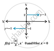
Domain= R and Range= {-1,0,1}

(vii) Greatest integer function- Greatest integer function are of type f(x)= [x]= greatest integer less than or equal to x.
Try to understand it by taking few values of x
x= (2.1), f(2.1)= [2.1]= 2
x= (3.9), f(3.9)= [3.9]= 3
x= (-2.3), f(-2.3)= [-2.3]= -3
x=5, f(5)= [5]= 5

Domain= R and Range= Integers i.e Z