Methods of Measuring Price Elasticity of Demand

Methods of Measuring Price Elasticity of Demand :

1) Ratio or Percentage method :
Ratio method is developed by Prof. Marshall. According to this method, elasticity of demand is measured by dividing the percentage change in demand by the percentage change in price. Percentage method is also known as Arithmetic method. Price elasticity is measured as :

`"Ed" = "Percentage change in Quantity demanded"/"Percentage change in Price"`

`"Ed"="%ΔQ"/"%ΔP"`

Mathematically, the above formula can be presented as under.

`"Ed"="ΔQ"/"Q"÷"ΔP"/"P"`

∴ `"Ed" = "ΔQ"/"Q"xx"P"/"ΔP"`

Q = Original quantity demanded
ΔQ = Difference between the new quantity and original quantity demanded.
P= Original price
ΔP= Difference between new price and original price

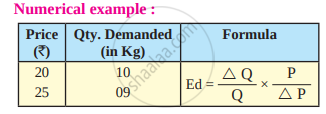
Original Price, P = 20, New price P = 25
ΔP = 5 (Difference between new and original price)
Original Quantity Demanded, Q = 10, New demand = 9
ΔQ = 1 (Difference between new and original quantity demanded)

`"Ed" = "ΔQ"/"Q"xx"P"/"ΔP"`

`"Ed"="1"/"10"xx"20"/"5"`

Ed= 0.4

Ed < 1

It means elasticity of demand is relatively inelastic.

2) Total Expenditure Method :
This method was developed by Prof. Marshall. In this method, total amount of expenditure before and after the price change is compared.
 Here the total expenditure refers to the product of price and quantity demanded.

In this connection, Marshall has given the following propositions :
A) Relatively elastic demand (Ed >1) :
When with a given change in the price of a commodity total outlay increases, elasticity of demand is greater than one.
B) Unitary elastic demand (Ed = 1) :
When price falls or rises, total outlay does not change or remains constant, elasticity of demand is equal to one.
C) Relatively inelastic demand (Ed <1) :
When with a given change in price of a commodity total outlay decreases, elasticity of demand is less than one.

In case ‘A’, original price is ₹6 per unit and quantity 5 per unit demanded is 10 units. Therefore, total expenditure incurred is ₹60. When price falls to ₹ 5 quantitydemanded rises to 20 units, the total expenditure incurred is ₹100. In this case, total outlay is greater than original expenditure. Hence, at this stage, elasticity of demand is greater than one. (Ed >1) that is relatively elastic demand.
In case ‘B’, original price is ₹4 per unit and quantity demanded is 30 units. Therefore total expenditure is ₹120. When price falls to ₹‘3’ per unit quantity demanded rises to 40 units. Total expenditure incurred is ₹120. In this case total outlay is same (equal) to original expenditure. Hence, at this point, elasticity of demand is equal to one (Ed = 1) that is unitary elastic demand.
In case ‘C’, original price is ₹2 per unit and quantity demanded is 50 units. Therefore total expenditure is ₹100. When price falls to ₹1 per unit, quantity demand rises to 60 unit and total expenditure incurred is ₹60. In this case total outlay is less than original expenditure. 
Hence, elasticity of demand is less than one (Ed <1) that is relatively inelastic demand.

3) Point method or Geometric Method :
Prof. Marshall has developed another method to measure elasticity of demand, which is known as point method or geometric method. The ratio method and total outlay methods are unable to measure elasticity of demand at a given point on the demand curve.
At any point on the demand curve, elasticity of demand is measured with the help of the following formula :

`"Point elasticity of demand (Ed)"="Lower segment of demand curve below a given point (L) "/"Upper segment of demand curve above a given point (U)"`

Demand curve may be either linear or non-linear as shown below :

A) Linear Demand Curve :
When the demand curve is linear i.e. a straight line, we extend the demand curve to meet the Y axis at ‘A’ and X axis at ‘B’. Price elasticity of demand at ‘X’ axis is zero and ‘Y’ axis is infinite. Elasticity of demand will be different at each point.

Let us assume that AB is a demand curve and its length is 8 cm. Point elasticity at various points on a linear demand curve can be measured as follows :

1) At point P, the point elasticity is measured as :

`"P"="PB"/"PA"="4"/"4"=1"`

Thus, at point P, demand is unitary elastic (ed = 1)

2) At point P₁ , the point elasticity is measured as :

`"P"_"1"=("P"_1"B")/("P"_1"A")="2"/"6"=0.33"`

Thus, at point P1 , demand is relatively inelastic (ed < 1)

3) At point P2 , the point elasticity is measured as :

`"P"_"2"=("P"_2"B")/("P"_2"A")="6"/"2"=3`

Thus, at point P2 , demand is relatively elastic (ed > 1)

4) At point A, the point elasticity is ∞ (perfectly elastic demand)
5) At point B, the point elasticity is zero (perfectly inelastic demand.)

B) Non-linear demand curve :
When the demand curve is non-linear i.e. convex to origin, to measure price elasticity of demand we have to draw a tangent ‘AB’ touching the given point on the demand curve and extending it to meet ‘Y’ axis at point ‘A’ and ‘X’ axis at point ‘B'.

`"Ed" = "Lower segment of the tangent below a given point"/"Lower segment of the tangent below a given point"="L"/"U"`

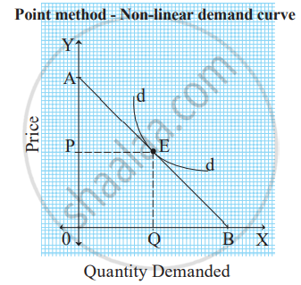
If EB = EA (Ed = 1) - Unitary elastic demand
EB > EA (Ed >1) - Relatively elastic demand
EB < EA (Ed <1) - Relatively inelastic demand