Geometrical Meaning of the Zeroes of a Polynomial

1)  In a general, given a polynomial p(x) of degree n, the graph of y=p(x) intersects the x-axis at atmost n points. Therefore, a polynomial p(x) of degree n has at most n zeroes.
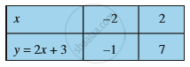
Example- Consider first a linear polynomial ax + b, a ≠ 0. You have studied in Class IX that the graph of y = ax + b is a straight line. For example, the graph of y = 2x + 3 is a straight line passing through the points (– 2, –1) and (2, 7).

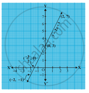 From Fig. you can see that the graph of y = 2x + 3 intersects the x-axis mid-way between x = –1 and x = – 2,
that is, at the point `(-3/2,0)`
You also know that the zero of
2x + 3 is `-3/2`
Thus, the zero of the polynomial 2x + 3 is the x-coordinate of the point where the graph of y = 2x + 3 intersects the x-axis.
2)Any polynomial of odd degree will never have nil zeroes. Polynomials with odd degree of power will have minimum one 0.  Whereas polynomials having even degree of power have minimum zero 0.
Example1- Let us see what the graph of a even polynomial  `y = x^2 – 3x – 4` looks like. Let us list  a few values of `y = x^2 – 3x – 4` corresponding to a few values for x as given in Table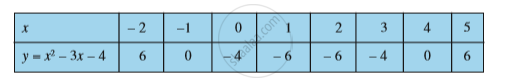

If we locate the points listed above on a graph paper and draw the graph, it will actually look like the one given in Fig.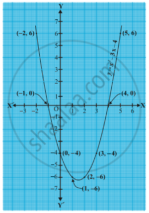

In fact, for any quadratic polynomial `ax2 + bx + c,` a ≠ 0, the graph of the corresponding equation y = `ax^2 + bx + c` has one of the two shapes either open upwards like  or open
downwards like  depending on whether a > 0 or a < 0. (These curves are called parabolas.)
You can see from Table that –1 and 4 are zeroes of the quadratic polynomial. Also note from Fig that –1 and 4 are the x-coordinates of the points where the graph of `y = x2 – 3x – 4 ` intersects the x-axis. Thus, the zeroes of the quadratic polynomial `x^2 – 3x – 4` are x-coordinates of the points where the graph of `y = x^2 – 3x – 4` intersects the x-axis.
Example2-  Consider a odd polynomial `x^3 – 4x`. To see what the graph of `y = x^3 – 4x` looks like, let us list a few values of y corresponding to a few values for x as shown in Table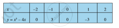 

Locating the points of the table on a graph paper and drawing the graph, we see that the graph of `y = x^3 – 4x` actually looks like the one given in Fig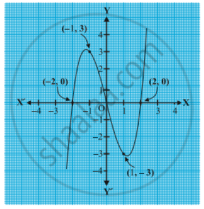

We see from the table above that – 2, 0 and 2 are zeroes of the cubic polynomial `x^3 – 4x`. Observe that –2, 0 and 2 are, in fact, the x-coordinates of the only points where the graph of `y = x^3 – 4x` intersects the x-axis. Since the curve meets the x-axis in only these 3 points, their x-coordinates are the only zeroes of the polynomial.