Topics
Matter in Our Surroundings
- Matter (Substance)
- Characteristics of Particles (Molecules) of Matter
- The Solid State
- The Liquid State
- The Gaseous State
- Plasma
- Bose-einstein Condensate
- Heat and change of physical state
- Concept of Evaporation
- Concept of Melting (Fusion)
- Concept of Boiling (Vaporization)
- Concept of Sublimation
- Concept of Freezing (Solidification)
- Concept of Condensation (Liquefaction)
- Concept of Desublimation (Deposition)
Is Matter Around Us Pure
- Matter (Substance)
- Natural substances
- Mixture
- Types of Mixtures
- Solution
- Concentration of a Solution
- Suspension Solution
- Colloidal Solution
- Evaporation Method
- Solvent Extraction (Using a Separating Funnel Method)
- Sublimation Method
- Chromatography Method
- Simple Distillation Method
- Fractional Distillation Method
- Crystallisation Method
- Classification of Change: Physical Changes
- Chemical Reaction
- Pure Substances
- Compound
- Elements
Atoms and Molecules
- History of Atom
- Laws of Chemical Combination
- Law of Conservation of Mass
- Law of Constant Proportions (Law of Definite Proportions)
- Dalton’s Atomic Theory
- Atoms: Building Blocks of Matter
- Symbols Used to Represent Atoms of Different Elements
- Atomic Mass
- Relative Atomic Mass (RAM)
- Molecules
- Classification of Molecules
- Difference Between Atoms and Molecules
- Ions (Radicals) and Its Types
- Chemical Formula or Molecular Formula
- Molecular Mass
- Formula Unit Mass
- Mole Concept
- Atoms and Molecules Numericals
Structure of the Atom
- Existence of Charged Particles in Matter
- Atoms: Building Blocks of Matter
- Discovery of Charged Particles in Matter
- Protons (p)
- Electrons (e)
- Neutrons (n)
- J. J. Thomson’s Atomic Model
- Advantage and Limitations of Thomson’s Atomic Model
- Lord Rutherford’s Atomic model
- Limitations of Rutherford’s Atomic Model
- Neils Bohr’s Model of an Atom
- Electronic Configuration of Atom
- Valency
- Different Ways to Determine Valency
- Atomic Number (Z), Mass Number (A), and Number of Neutrons (n)
- Atomic Mass
- Isotopes
- Uses of Radioactive Isotopes
- Isobars
- Atoms and Molecules Numericals
The Fundamental Unit of Life
- Cell: Structural and Functional Unit of Life
- The Invention of the Microscope and the Discovery of Cell
- Cell Theory
- Organisms Show Variety in Cell Number, Shape and Size
- Prokaryotic and Eukaryotic Cell
- Simple Diffusion
- Concept of Osmosis
- Osmotic Pressure
- Structure of the Cell
- Plasma Membrane
- Semi-permeable Membrane (Cell Membrane)
- Cell Wall - “Supporter and Protector”
- Nucleus - “Brain” of the Cell
- Cytoplasm - “Area of Movement”
- Endoplasmic Reticulum (ER)
- Golgi Apparatus - "The delivery system of the cell"
- Lysosome - “Suicidal Bag”
- Mitochondria - “Power House of the Cell”
- Plastids
- Non-living Substances Or Cell Inclusion
- Plant Cell and Animal Cell
- Cell Division: an Essential Life Process
Tissues
- Tissues - “The Teams of Workers”
- Plant and Animals Tissue
- Plant Tissues
- Meristems or Meristematic Tissues
- Permanent Tissue
- Simple Permanent Tissues (Supporting Tissue)
- Complex Permanent Tissues
- Complex Permanent Tissue: Xylem Structure and Function (Conducting Tissue)
- Complex Permanent Tissue: Phloem Structure and Function (Conducting Tissue)
- Animal Tissues
- Epithelial Tissue
- Connective Tissue
- Muscular Tissue
- Nervous Tissue
Motion
- Motion and Rest
- Describing Motion
- Motion Along a Straight Line
- Types of Motion
- Measuring the Rate of Motion - Speed with Direction
- Rate of Change of Velocity
- Distance and Displacement
- Displacement - Time Graph Or Distance - Time Graph
- Velocity - Time Graphs
- Equations of Motion by Graphical Method
- Derivation of Velocity - Time Relation by Graphical Method
- Derivation of Displacement - Time Relation by Graphical Method
- Derivation of Displacement - Velocity Relation by Graphical Method
- Uniform Circular Motion (UCM)
- Motion (Numerical)
Diversity in Living Organisms
- Biodiversity
- Biological Classification
- Classification of Living Organisms
- Taxonomic Hierarchy of Living Organisms: Unit of Classification
- Five Kingdom Classification
- Kingdom Monera
- Kingdom Protista
- Kingdom Fungi
- Classification of Kingdom Plantae
- Kingdom Animalia
- Differences Between Plantae (Plants) and Animalia (Animals)
- Classification of Kingdom Plantae
- Kingdom Plantae: Thallophyta (Algae)
- Kingdom Plantae: Thallophyta (Fungi)
- Division II- Bryophytes
- Division III- Pteridophytes
- Division I-Gymnosperms
- Division II- Angiosperms
- Kingdom Animalia
- Phylum: Porifera
- Phylum: Cnidaria/Coelenterata
- Phylum: Platyhelminthes
- Invertebrate: Phylum Nematoda
- Phylum: Annelida
- Phylum: Arthropoda
- Phylum: Mollusca
- Phylum: Echinodermata
- Subphylum: Prochordata
- Chordata: Vertebrata
- Invertebrata and Vertebrata
- Taxonomy and Systematics
- Nomenclature
Force and Laws of Motion
Gravitation
Work and Energy
Sound
- Sound
- Production of Sound
- Propagation of Sound
- Sound Need a Medium to Travel
- Sound Waves Are Longitudinal Waves
- Characteristics of a Sound Wave
- Speed of Sound (Velocity of Sound)
- Reflection of Sound
- Echoes
- Reverberation
- Uses of Multiple Reflection of Sound
- Range of Hearing in Humans
- Ultrasonic Sound Or Ultrasound
- SONAR
- Human Ear
- Sound (Numerical)
Improvement in Food Resources
- Improvements in Food Resources
- Improvement in Crop Yields
- Crop Variety Improvement
- Crop Production Improvement
- Crop Protection Management
- Methods to Replenish Nutrients in Your Soil
- Manuring (Biomanuring)
- Fertilizers
- Improved methods of agriculture
- Agricultural Assistance Programme
- Animal Husbandry (Livestock)
- Dairy Farming
- Poultry Farming
- Pisciculture (Fish Farming)
- Apiculture (Bee Farming)
Why Do We Fall ill
- Health
- Disease
- Categories of Disease
- Acute and Chronic Diseases
- Causes of Disease
- Communicable Or Infectious Diseases
- Infectious Agents
- Manifestation of Diseases
- Modes of Transmission of Diseases
- Organ-specific and Tissue-specific Manifestations
- Principles of Prevention of Diseases
- Principles of Treatment of Diseases
Natural Resources
- Natural Resources
- Biosphere: The Domain of Life
- Air is a Mixture
- Atmosphere and Its Layers
- Wind: The Movement of Air
- Rain
- Water: Our Lifeline
- Where Do We Get Water From?
- Availability of Water
- Importance of Water
- Water Pollution and Its Causes
- Mineral Riches in the Soil
- Biogeochemical Cycle
- Water Cycle
- Nitrogen Cycle
- The Carbon Cycle
- The Oxygen Cycle
- Ozone
- Ozone Layer Depletion
- Velocity-time graph for uniform velocity
- Velocity-time graph for uniform acceleration
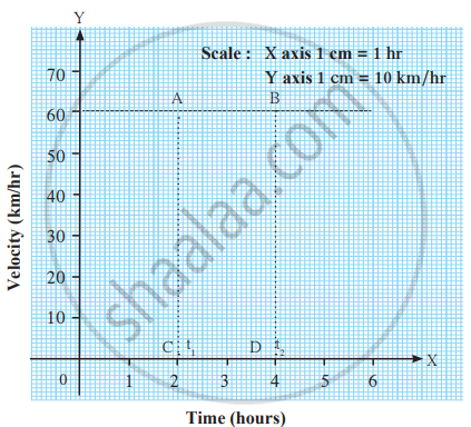
Velocity-Time Graph for Uniform Velocity
Activity:
The train moves at a constant velocity of 60 km/h for 5 hours, which means the velocity remains the same throughout.
- To determine the distance covered between 2 and 4 hours, look at the area under the velocity-time graph between these two time points.
- The area under a velocity-time graph represents the distance travelled. In this case, it's a rectangle because the velocity is constant.
- The distance covered between 2 and 4 hours is equal to the area of the rectangle formed by the velocity of 60 km/h and the time interval from 2 to 4 hours.
The formula for distance is Distance = Velocity × Time.
In this case, Distance = 60 km/h × (4 - 2) hours = 60 × 2 = 120 km.
Since the train is moving at uniform velocity, there is no acceleration. Acceleration is zero because the speed doesn't change over time.
Velocity-time graph
Velocity-Time Graphs:
To draw velocity-time graphs, we will use the three equations of motion.
Case 1: Velocity-time graphs with constant velocity (zero acceleration)
When the velocity is constant, the velocity-time graph, with the Y-axis denoting velocity and the X-axis denoting time, will be like:
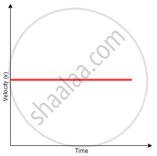
The graph clearly shows that the velocity remains constant at c throughout the time interval. No particles of matter how much the time changes, the velocity will be c at every instant. In this case, we have taken the initial velocity to be positive. The graph will be different if the initial velocity is negative.
Example: If the acceleration of a particle is zero (0), and velocity is constantly, say, 5 m/s at t = 0, then it will remain constant throughout the time.
Case 2: Velocity-time graphs with constant acceleration
When the acceleration is constant (positive), and the initial velocity of the particle is zero, the velocity of the particle will increase linearly as predicted by the equation:
v = u + at
Since u = 0
v = at
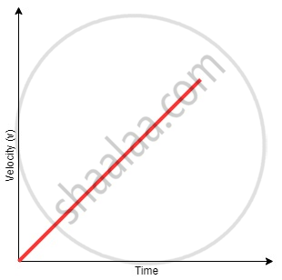
As shown in the figure, the velocity of the particle will increase linearly with respect to time. The slope of the graph will give the magnitude of acceleration.
Example: If the acceleration of a particle is constant (k) and is positive, the initial velocity is zero, and then the velocity increases linearly. The slope of the velocity-time graph will give the acceleration.
Case 3: Velocity-time graphs with increasing acceleration
When the acceleration is increasing with time, the velocity-time graph will be a curve as predicted from the equation:
v = u + at
Since u = 0
v= at
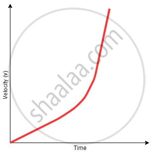
Since acceleration is a function of time, the velocity-time graph will be a curve.
Note: Since the acceleration is continuously increasing with time, the magnitude of the slope will also continuously increase with time.
When an object moves along a straight line with uniform acceleration, it is possible to relate its velocity, acceleration during motion and the distance covered by it in a certain time interval by a set of equations known as the equations of motion. For convenience, a set of three such equations is given below:
v = u + at ......(1)
s = `"ut" + 1/2at^2` ......(2)
`2 as = "v"^2 – "u"^2` ......(3)
where u is the initial velocity of the object that moves with uniform acceleration a for time t, v is the final velocity, and s is the distance travelled by the object in time t. Eq. (1) describes the velocity-time relation and Eq. (2) represents the position-time relation.
Eq. (3), which represents the relation between the position and the velocity, can be obtained from Eqs. (1) and (2) by eliminating t.
These three equations can be derived by graphical method.
Velocity-Time Graph for Uniform Acceleration:
The table shows the velocity of the car at different times, increasing by 8 m/s every 5 seconds. This means the car is accelerating uniformly, and the velocity increases by equal amounts in equal time intervals.
The velocity change every 5 seconds is 8 m/s, so in 5 minutes (300 seconds), the total change in velocity would be:
- Number of 5-second intervals = `"300"/"5"`=60
- Total velocity change = 60 × 8 = 480 m/s.
The velocity-time graph is a straight line because the car is uniformly accelerating. In non-uniformly accelerated motion, the graph would be curved, showing varying acceleration over time.
To calculate the distance covered between the 10th and 20th seconds, we need to find the average velocity in that interval.
The average velocity is the mean of the velocities at 10 seconds (16 m/s) and 20 seconds (32 m/s), which is `"16+32"/"2"`=24 m/s.
The distance is then:
Distance = Average velocity × Time = 24 × 10 = 240
Check that, similar to the example of the train, the distance covered is given by the area of quadrangle ABCD.
The area can be split into two parts:
1. Rectangle AECD
Base = 10 seconds (from 10s to 20s)
Height = 16 m/s (velocity at 10 seconds)
Area = 10×16=160 m
2. Triangle ABE
Base = 10 seconds (time from 10s to 20s)
Height = 16 m/s (difference in velocity from 16 m/s to 32 m/s)
Area = 12×10×16 = 80 m
Total distance = Area of rectangle + Area of triangle = 160 m + 80 m = 240 m.
The total area of quadrangle ABCD gives the distance travelled, confirming the calculation.
| Time (seconds) | Velocity (m/s) |
|---|---|
| 0 | 0 |
| 5 | 8 |
| 10 | 16 |
| 15 | 24 |
| 20 | 32 |
| 25 | 40 |
| 30 | 48 |
| 35 | 56 |

Velocity-time graph
Shaalaa.com | Velocity Time Graph
Related QuestionsVIEW ALL [114]
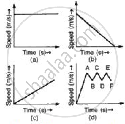
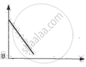
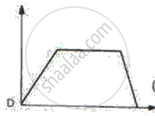
Given below are the speed -time graphs. Match them with their corresponding motions :
 |
(a) Uniformity retared motion |
 |
(b) Non-uniformity acceleration |
 |
(c) Non-uniform motion |
 |
(d) uniform motion |